Why Is My Vlookup Not Working When There Is A Match

I execute vlookup function in order to fill in 3 columns from table2 into table1. That's why you're using the approximate match setting to start with.

How To Use Vlookup And Match Formulas In Excel

For my case, the lookup value is not a value that i insert as input, but a formula.

Why is my vlookup not working when there is a match. For example in a1=1 and a2=a1+1. When vlookup formula cannot find a match, then this error displays, meaning “not available.” but it is always not correct that the lookup value is actually not available. The problem that i keep getting however is that if the result of the vlookup is a cell with a hyperlink, the hyperlink does not work.

In that case, excel moves through the lookup values in the table until it. In the function arguments window, check the lookup_value and table_array values text values are wrapped with quote marks; Same conditions also apply for the rest of the.

So if you were looking for abc, then it would ignore 123abc456. Vlookup with an approximate match works completely different from exact match which is why you should always stick to using the exact match. This is one of the most common reasons behind the #na error in vlookup.

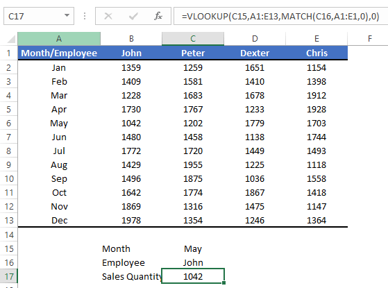
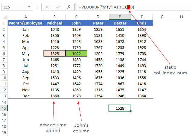
First, when you're using vlookup for approximate matches, it's likely that the lookup value won't be in the table. Select the vlookup formula cell, and click the fx button in the formula bar. Now, even if columns are inserted and the column for bonus is changed, our formula will adapt with the change and still return the correct column number.

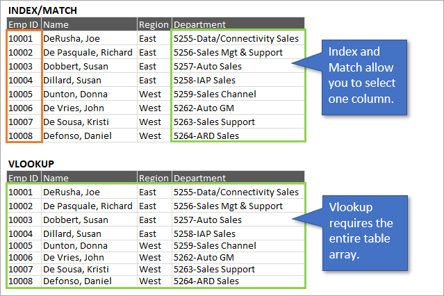
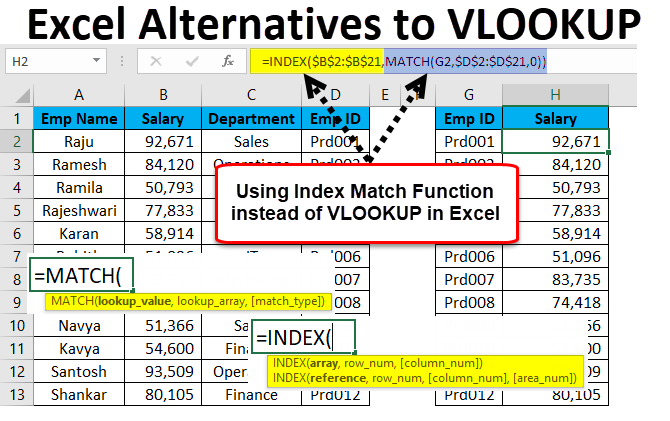
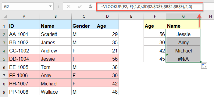
Tried to mess around with =hyperlink(vlookup) but it also doesn’t seem to work. You can use 0 (the number zero) which technically is the same as false. Index match combines two functions in excel and allows you to actually select the column you want to return values from manually with your mouse.

A zero formatted as a date returns 01/01/1900 as this is the starting date used by excel. If you are working on multiple column data, it’s a pain to change its reference because you have to do this manually. The quick way to test is to select cell a2 and press the f2 key to put the cell in edit mode.

However, there are some few exceptions. There are some constraints with it, though, for example, you must name a single number to indicate the column that will be returning values. I made sure that both columns (for comparison) have the same format (general) and there is no extra spacing.

Vlookup not detecting text matches problem: Extra spaces in lookup value. The approximate match returns the next largest value that is less than your specific lookup value.

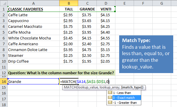
When the range_lookup argument is false—and vlookup is unable to find an exact match in your data—it returns the #n/a error. If match_type is 0 and lookup_value is text, the wildcard characters question mark. Why my vlookup function does not work?

In practice, we often forget about this and end up with vlookup not working because of the n/a error. Vlookup looks for a cell that matches in the entire cell. The vlookup/match function is not behaving normal when i am looking for a2 in a table,.sometimes it shows the n/a error and sometimes it works.

With b4 mentioning the vendor number in my new table. Match returns the #n/a error if no match is found the argument lookup_array must be placed in descending order: Whenever i encounter a vlookup or match function failing, my first impulse is that one cell has trailing spaces.

Use the =trim formula on both corresponding columns (and then remove formulas) to make sure all cells in both corresponding columns are text fields. The best way to solve this problem is to use match function in vlookup for col_index_number. All or some of the cells in either of the corresponding columns aren't being recognized as a text field/cell.

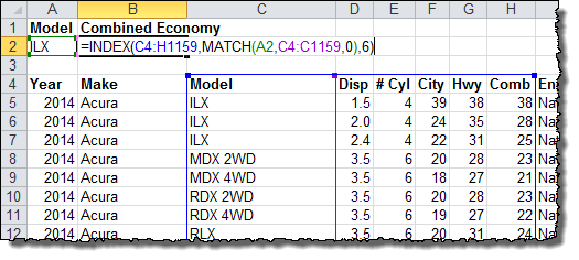
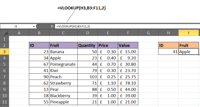
For some reason, the formula doesn't work for the first row, and doesn't find the exact match from table2 even though it exists. D2 is the value which you want to return its relative information, a2:b10 is the data range you use, the number 2 indicates the column number that your matched value is returned and the true refers to the approximate match. The most common reason this happens though is due to leading or trailing spaces.

I have an issue with the vlookup/match. The issue revolves around the use of 15 & 015, which is to the right of 'abc' in my table below. Although humans don’t see spaces as characters, a space is a character in excel.

To make the vlookup formula work correctly, the values have to match. Also, ensure that the cells follow the correct. There could be some reasons why vlookup returns this error.

In vlookup, col_index_no is a static value which is the reason vlookup doesn’t work like a dynamic function. In big data set it is very hard to identify. Sorting the data in sheet1 by the date column (column e) by largest to smallest should do the trick.

Real number have no quote marks;

Excel Formula Partial Match With Vlookup Exceljet